Organization of disparity-selective neurons in macaque area MT

Abstract

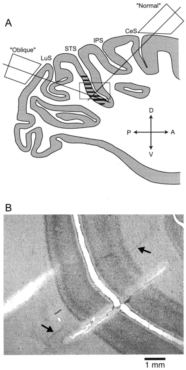
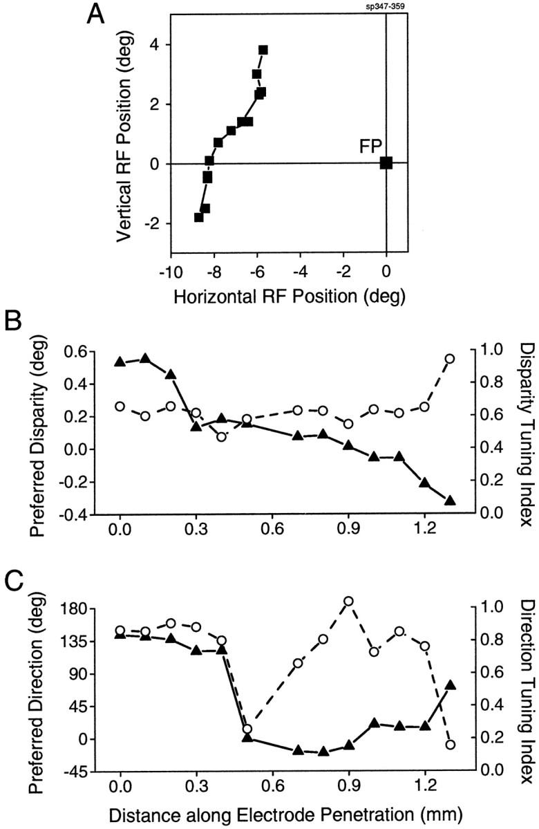
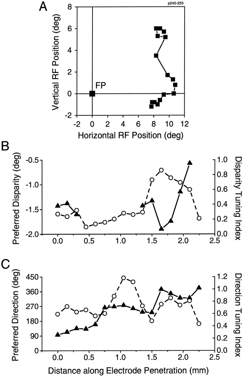
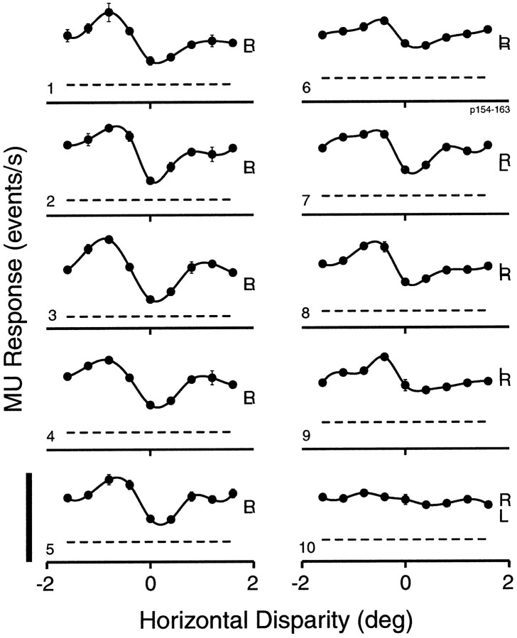
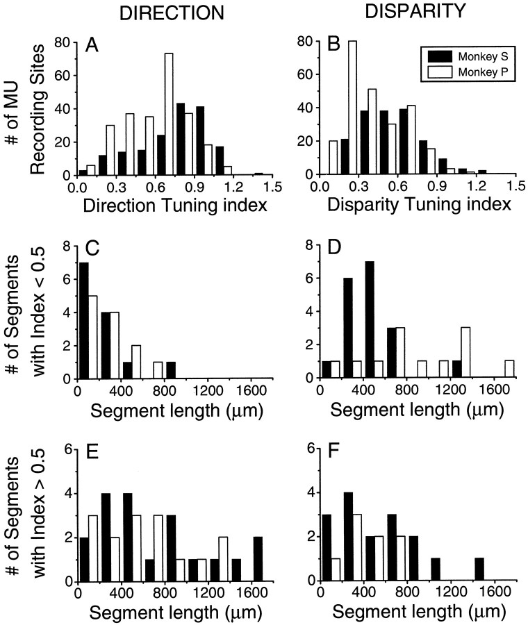
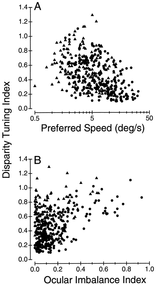
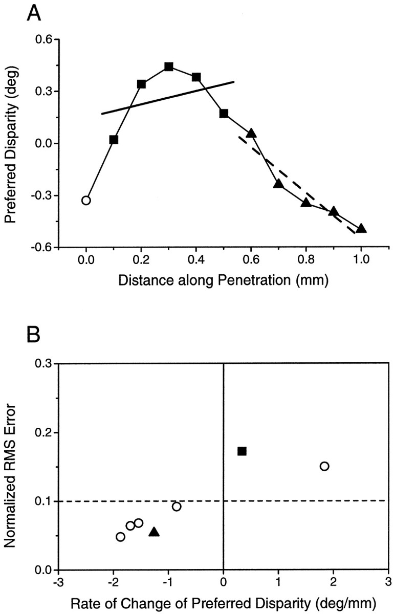
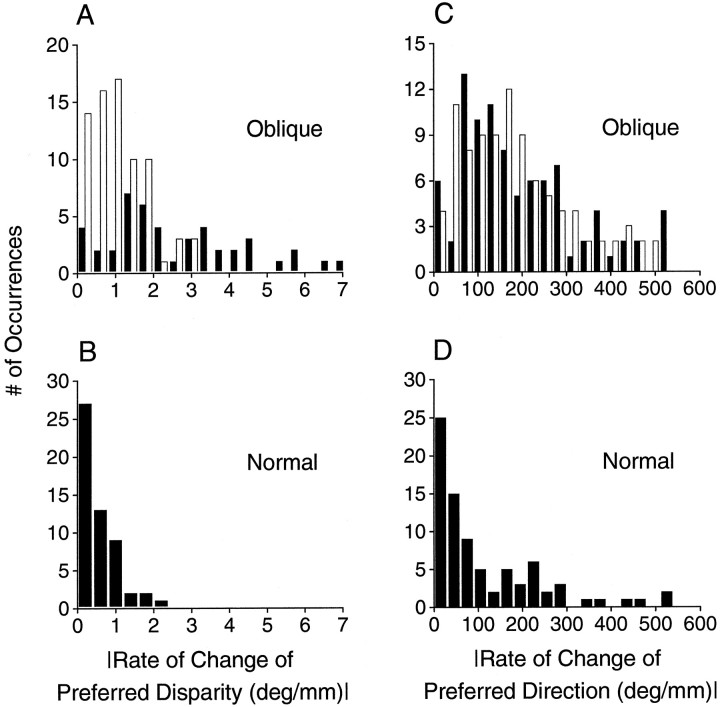
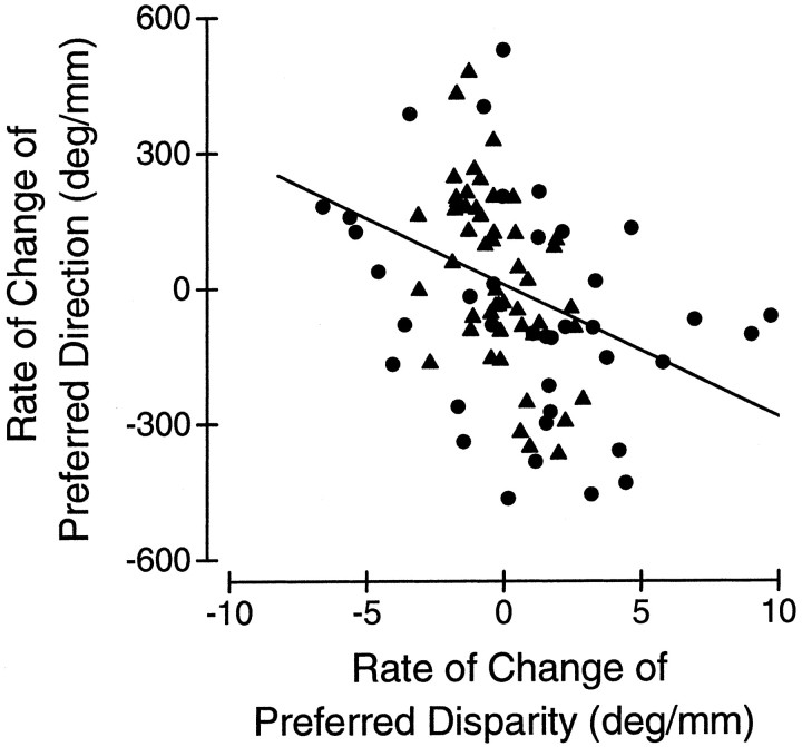
Neurons selective for binocular disparity are found in a number of visual cortical areas in primates, but there is little evidence that any of these areas are specialized for disparity processing. We have examined the organization of disparity-selective neurons in the middle temporal visual area (MT), an area shown previously to contain an abundance of disparity-sensitive neurons. We recorded extracellularly from MT neurons at regularly spaced intervals along electrode penetrations that passed through MT either normal to the cortical surface or at a shallow oblique angle. Comparison of multiunit and single-unit recordings shows that neurons are clustered in MT according to their disparity selectivity. Across the surface of MT, disparity-selective neurons are found in discrete patches that are separated by regions of MT that exhibit poor disparity tuning. Within disparity-selective patches of MT, we typically observe a smooth progression of preferred disparities (e.g. , near to far) as our electrode travels parallel to the cortical surface. In electrode penetrations normal to the cortical surface, on the other hand, MT neurons generally have similar disparity tuning, with little variation from one recording site to the next. Thus disparity-tuned neurons are organized into cortical columns by preferred disparity, and preferred disparity is mapped systematically within larger, disparity-tuned patches of MT. Combined with other recent findings, the data suggest that MT plays an important role in stereoscopic depth perception in addition to its well known role in motion perception.

Fig. 1.

Schematic illustration of the visual stimulus. The fixation point (FP) is indicated by a yellow cross. Moving dots of variable disparity were presented within a square aperture (dashed yellow lines) that was centered over and slightly larger than the receptive field (RF, white circle) of the recorded MT neurons. The white arrow denotes the direction of motion of the dots. Dotsrendered outside the plane of fixation are shown as horizontally disparate red and green pairs, in which the red dots indicate the left eye’s image and thegreen dots denote the right eye’s image. Yellow dots outside the square aperture were presented at zero disparity and provided a background.

Fig. 2.

Illustration of electrode penetrations through MT.A, Schematic diagram showing the locations of recording cylinders and the electrode approaches to MT. The drawing is of a sagittal section through the brain of a monkey not used in the present study; shaded regions indicate gray matter. Thehatched region of gray matter represents MT.Lines emerging from the recording cylinders (Normal and Oblique) indicate typical electrode trajectories from the two recording cylinders. For oblique penetrations, the recording cylinder was mounted over the occipital lobe at an angle 20° below the horizontal. For normal penetrations, the recording cylinder was mounted over the precentral gyrus at an angle 45° below the horizontal.A, Anterior; CeS, central sulcus;D, dorsal; IPS, intraparietal sulcus;LuS, lunate sulcus; P, posterior;STS, superior temporal sulcus; and V, ventral. B, Nissl-stained section from the right hemisphere of monkey P, which was implanted with the frontally located cylinder. The section depicts a midportion of the superior temporal sulcus, approximately equivalent to the rectangular boxin A, in a near-sagittal plane. The two largescars were made by marking pins that were implanted just before perfusion along the trajectory of the normal microelectrode penetrations. Faint scars from microelectrode penetrations are also visible (arrows). Scale bar, 1 mm.

Fig. 3.

An example data set from one recording site.A, Direction-tuning curve. Filled circlesshow the mean multiunit (MU) response (± 1 SE) to eight different directions of motion, 45° apart. Each direction was presented four times, and trials were block randomized. The solid curve is the best-fitting Gaussian.R_max and R_mindenote the maximum and minimum values of the Gaussian curve. Thedashed line represents the spontaneous activity level (S). The preferred direction (Pref. Dir.) is defined as that at which the Gaussian has its peak.B, Disparity-tuning curve. Conventions are as described in A, except that the solid curve is a cubic spline interpolation. Filled symbols labeledL and R (right) indicate the responses obtained during monocular controls when dots were presented to only the left or right eye, respectively.C, Area-summation curve. The solid curvehere is the best fit of a difference of two error functions (see text for details). Optimal size (Opt. Size) is that at which the smooth curve has its peak, and percent surround inhibition measures the attenuation of the response at large sizes relative to the peak response. The response at size zero is equivalent to spontaneous activity.

Fig. 4.

Comparison of disparity-tuning curves recorded simultaneously from single-unit spikes (open circles;right y-axis) and multiunit activity (filled circles; left y-axis) at six representative sites in MT. The smooth curves in each panel were generated by cubic spline interpolation. Each datum is the mean of four or five stimulus repetitions, and error bars indicate SE. The solid and dashed horizontal lines denote the spontaneous activity levels for multiunit (MU) and single-unit (SU) responses, respectively. Symbols L and Rdenote responses to the same moving random-dot pattern when presented monocularly to either the left or right eye, respectively.A, Both MU and SUresponses exhibiting sharp disparity tuning to a narrow range of near (i.e., negative) disparities. Eccentricity (Ecc.) = 7.4°; RF diameter (RF diam.) = 9°; preferred disparity (PD) = −0.36° (MU) or −0.37° (SU); and disparity-tuning index (DTI) = 1.1 (MU) or 1.25 (SU). B, Responses at a typical tuned-far site. Ecc. = 6.8°; RF diam. = 7.5°; PD = 0.58° (MU) or 0.50° (SU); and DTI = 0.53 (MU) or 0.80 (SU). C, Responses at a typical tuned-near site. Ecc. = 5.6°; RF diam. = 7°; PD = −0.07° (MU) or −0.08° (SU); and DTI = 0.62 (MU) or 1.17 (SU). D, Responses at a site with broad selectivity for far disparities. Ecc. = 8.6°; RF diam. = 7.5°; PD = 0.52° (MU) or 0.49° (SU); and DTI = 0.89 (MU) or 1.03 (SU).E, Both MU and SU at this site responsive over a broad range of near disparities. Ecc. = 10.2°; RF diam. = 11°; PD = −0.73° (MU) or −1.6° (SU); and DTI = 0.56 (MU) or 0.96 (SU).F, At this site, both MU andSU responses exhibiting very weak disparity tuning. Ecc. = 8.4°; RF diam. = 8°; and DTI = 0.14 (MU) or 0.22 (SU).

Fig. 5.

Quantitative comparison of disparity- and direction-tuning parameters derived from multiunit (MU) and single-unit (SU) responses. In each panel, data from SUsare plotted on the y-axis, and data fromMU activity are plotted on the x-axis.Circles and triangles represent data from monkeys P and S, respectively. The solid line is the identity line, and the dashed line is the best linear fit to the data (linear regression). A, Comparison of disparity-tuning indices. B, Comparison of preferred disparities. C, Comparison of direction-tuning indices.D, Comparison of preferred directions.

Fig. 6.

Sequence of disparity-tuning curves recorded along an oblique penetration through MT in monkey S. Curves arenumbered in the order in which they were obtained. Each graph shows multiunit (MU) response plotted against horizontal disparity. Dashed horizontal linesrepresent the spontaneous activity level at each site, andletters L and R are plotted at the response levels measured in monocular controls. Error bars indicate SE and are plotted around each mean but are generally smaller than the data points themselves. Scale bar, 400 events/sec.

Fig. 7.

Quantitative summary of data recorded along the same oblique penetration illustrated in Figure 6. A, Location of the center of the MU receptive field (RF) at each recording site. RFlocation was estimated using a computerized search program (see Materials and Methods) and is plotted relative to the fixation point (FP) that has coordinates (0,0). The sequence ofRF locations begins in the lower left quadrant and moves upward toward thehorizontal meridian. B, Changes in disparity tuning quantified by plotting the disparity-tuning index (open circles; right y-axis) and the preferred disparity (filled triangles;left y-axis) as a function of distance along the electrode penetration. Note that preferred disparities are not plotted for sites where disparity tuning was not statistically significant (ANOVA, p > 0.05). C, Quantitative summary of changes in direction tuning. Direction-tuning index (open circles; right y-axis) and preferred direction of motion (filled triangles;left y-axis) are plotted in the same format used inB.

Fig. 8.

Quantitative data summary for another oblique penetration from monkey S. The format of this figure is identical to that of Figure 7.

Fig. 9.

Quantitative data summary for an oblique penetration from monkey P. Note that the disparity tuning is very weak for >1 mm at the beginning of the penetration, after which there is a region of strong disparity selectivity. The format of this figure is identical to that of Figure 7.

Fig. 10.

Sequence of disparity-tuning curves recorded at 150 μm intervals along a normal penetration from monkey P. Conventions are described in Figure 6. Note that almost all disparity-tuning curves have a very similar shape, with a preference for near disparities. Scale bar, 400 events/sec.

Fig. 11.

Quantitative data summary for the normal penetration of Figure 10. The format of this figure is identical to that of Figure 7.

Fig. 12.

Quantitative summary of the functional organization of disparity, direction, and speed tuning in MT. In eachpanel, circles are data derived from oblique penetrations, and triangles are data from normal penetrations. Filled symbols correspond to the parameter plotted on the left y-axis; open symbolscorrespond to the parameter plotted on the right y-axis.A, Filled circles andtriangles show the average absolute difference in preferred disparity ‖Δ Preferred Disparity‖ between pairs of recording sites as a function of distance between the sites. The solid horizontal line gives the value of ‖Δ Preferred Disparity‖ expected from drawing random pairs of sites from the entire population. Open circles andtriangles show the analogous data for preferred direction of motion ‖Δ Preferred Direction‖. The dashed horizontal line gives the value of ‖Δ Preferred Direction‖ expected from random pairings. The left andright y-axes have been scaled to round numbers so that the solid and dashed horizontal lines are approximately superimposed. B, Data are shown in the same format for the disparity-tuning index (filled symbols and solid horizontal line; left y-axis) and the direction-tuning index (open symbols and dashed horizontal line; right y-axis). C, Similar data are shown for the preferred speed of motion.

Fig. 13.

Analysis of the spatial organization of patches of weak and strong tuning for direction and disparity.A, Distribution of direction-tuning indices for monkey S (filled bars) and monkey P (open bars). All data shown in this figure are from multiunit (MU) recordings. B, Distribution of disparity-tuning indices. C, Distribution of lengths of penetration segments with poor direction tuning (direction-tuning index < 0.5). Only segments from oblique penetrations are included in this data set. D, Distribution of segment lengths with poor disparity selectivity (disparity-tuning index < 0.5). E, Histogram of segment lengths with strong direction tuning (direction-tuning index > 0.5).F, Histogram of segment lengths with strong disparity tuning (disparity-tuning index > 0.5).

Fig. 14.

Correlations of disparity-tuning index with other response parameters. A, Relationship between disparity-tuning index and preferred speed of motion. All data are derived from MU responses. Circles represent data from monkey P; triangles indicate data from monkey S. Note that preferred speed is plotted on a logarithmic axis.B, Relationship between disparity-tuning index and ocular imbalance index (OII, see Materials and Methods). OII is a measure of ocular dominance; small values denote matched response levels for the two eyes; large values indicate that one eye is dominant.

Fig. 15.

Method for computing rates of change of direction and disparity preference. A, Variation of preferred disparity with distance along an oblique penetration from monkey S. To measure slopes, we used a 400 μm sliding window (five data points) and performed linear regression on the data in this window. The window was then moved by one data point, and the process was repeated.Filled squares and triangles indicate two possible positions of the sliding window, and the solidand dashed straight lines show the best linear fits to data in these two windows. The open circle denotes a data point not included in either window. B, Normalized root-mean-square (RMS) error of the linear fit plotted as a function of the slope of the best-fitting line. The dashed horizontal line indicates an RMS error level of 0.1, which was our cut-off for accepting the linear fits. In this penetration, linear fits were accepted for five of seven positions of the sliding window, including the position denoted by the filled triangle. Two fits were rejected, including the one indicated by the filled square.

Fig. 16.

Summary of rates of change of preferred direction and disparity measured from oblique and normal penetrations. In each histogram, data from monkey S are indicated by open bars, and data from monkey P are denoted by filled bars. Note that these distributions give absolute values of the rates of change. A, Rates of change of preferred disparity in oblique penetrations. B, Rates of change of preferred disparity in normal penetrations. C, Rates of change of preferred direction in oblique penetrations.D, Rates of change of preferred direction in normal penetrations.

Fig. 17.

Comparison of signed rates of change in preferred direction and disparity. Triangles andcircles denote data from monkeys S and P, respectively. The solid line is the best linear fit (linear regression). Positive values on the y-axis correspond to preferred direction rotating counterclockwise; positive values on thex-axis correspond to preferred disparity changing from near to far.

Fig. 18.

Schematic summary of the functional architecture of MT, with regard to binocular disparity and direction of motion. Thetop surface of this slab corresponds to the surface of MT, and the height of the slab corresponds to the thickness of the cortex. Arrows denote the preferred direction of motion of MT neurons in each directioncolumn. Note that we have simply shown direction to vary smoothly across the surface of MT in both dimensions. We have not attempted to depict the direction map accurately, nor have we attempted to depict any discontinuities in the direction map (for comparison, seeMalonek et al., 1994). Preferred disparity is color-coded, withgreen representing near disparities, redrepresenting far disparities, and yellow indicating zero disparity. Dark blueregionsdenote portions of MT that have poor disparity tuning.

References

1. Albright TD. Direction and orientation selectivity of neurons in visual area MT of the macaque. J Neurophysiol. 1984;52:1106–1130. - PubMed
1. Albright TD. Cortical processing of visual motion. Rev Oculomotor Res. 1993;5:177–201. - PubMed
1. Albright TD, Desimone R. Local precision of visuotopic organization in the middle temporal area (MT) of the macaque. Exp Brain Res. 1987;65:582–592. - PubMed
1. Albright TD, Desimone R, Gross CG. Columnar organization of directionally selective cells in visual area MT of the macaque. J Neurophysiol. 1984;51:16–31. - PubMed
1. Barlow HB, Blakemore C, Pettigrew JD. The neural mechanism of binocular depth discrimination. J Physiol (Lond) 1967;193:327–342. - PMC - PubMed
Publication types
LinkOut - more resources