High dimensional predictions of suicide risk in 4.2 million US Veterans using ensemble transfer learning

Abstract

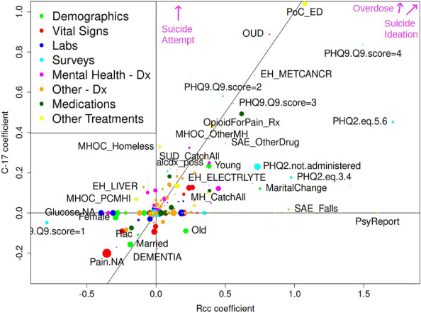
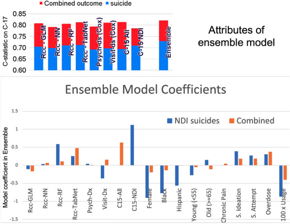
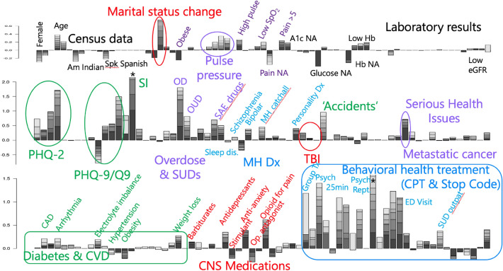
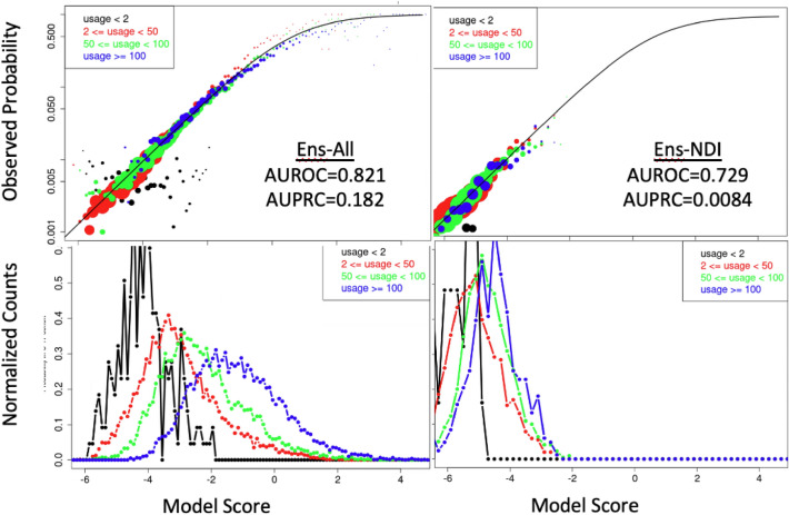
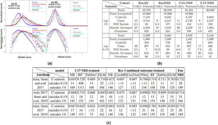
We present an ensemble transfer learning method to predict suicide from Veterans Affairs (VA) electronic medical records (EMR). A diverse set of base models was trained to predict a binary outcome constructed from reported suicide, suicide attempt, and overdose diagnoses with varying choices of study design and prediction methodology. Each model used twenty cross-sectional and 190 longitudinal variables observed in eight time intervals covering 7.5 years prior to the time of prediction. Ensembles of seven base models were created and fine-tuned with ten variables expected to change with study design and outcome definition in order to predict suicide and combined outcome in a prospective cohort. The ensemble models achieved c-statistics of 0.73 on 2-year suicide risk and 0.83 on the combined outcome when predicting on a prospective cohort of [Formula: see text] 4.2 M veterans. The ensembles rely on nonlinear base models trained using a matched retrospective nested case-control (Rcc) study cohort and show good calibration across a diversity of subgroups, including risk strata, age, sex, race, and level of healthcare utilization. In addition, a linear Rcc base model provided a rich set of biological predictors, including indicators of suicide, substance use disorder, mental health diagnoses and treatments, hypoxia and vascular damage, and demographics.

Figure 1

Three important aspects of study design for suicide prediction. At the top is a histogram of the first reported instance of each of the three related outcomes. The lack of deaths by suicide after 2018 is a result of a lag in available data from the National Death Index (NDI). At the bottom left is a diagram describing our retrospective case–control (Rcc) study design, with eight time windows of increasing width as the time before the outcome increases. At the bottom right is a diagram describing our four prospective cohorts, where our eight-time windows, defined as in Rcc, are aligned with a psychiatric visit (Cox-MH), an office visit (Cox-Visit), January 1, 2015 (C15), or January 1, 2017 (C17). Below the arrow are the numbers of patients with each outcome and the number of controls included in the cohort for Rcc (left) and C17 (right). Further details for all study designs are provided in the Methods section, and demographics are provided in Supplementary Table S2.

Figure 2

Comparison of model coefficients between Rcc and C17 logistic regression calculations. The x-axis designates the Rcc coefficients for each variable, while C17 coefficients are plotted along the y-axis, in both cases summed across the eight time bins. The area of the symbol is proportional to the number of cases with each variable present in at least one time bin, while the color is coded according to the category of variables, as described in the figure legend. The diagonal line is of slope one and can be used to assess the level of agreement in model coefficients across study designs. Suicide attempt (0.2, 5.1), suicide ideation (3.2, 1.7), and opioid overdose (1.8, 3.8) are indicated with arrows because they are off-scale.

Figure 3

Attributes of ensemble models: (top) C-statistic scores for eight base models and our ensemble models, fine-tuned for both the combined (red bars) and suicide (blue bars) outcomes, all evaluated for the C17 cohort. (bottom) Logistic regression coefficients define the ensemble model component amplitudes and their fine-tuning to predict outcomes for the C17 cohort. The eight left-most coefficients define each base model’s contribution to the ensemble and typically span a range of five units. The ten coefficients to the right define the contributions of the other variables used in the fine-tuning process. Nine of these are binary (0/1) variables, and usage ranges from 0 to 100 and is multiplied by 100 in this plot for ease of comparison. The models were fine-tuned with logistic regression and without cross-validation or model selection. More details of the fine-tuning process are provided in the Methods section.

Figure 4

Model coefficients for the Rcc study design and the logistic regression model predicting our combined outcome. Stacked bar charts indicate model coefficients, with darker shades indicating acute predictors (proximal to the event in Fig. 1), and lighter colors from time bins 3–7 years earlier. Upward direction indicates variables that are predictive of outcome events. The * above suicide ideation and psychiatric report indicate off-scale values of 3.2 and 1.6, respectively. Values of coefficients, prevalence, and other attributes are provided in Supplementary Table S3 for selected predictors. Individual labels are omitted from the figure, but the names of all coefficients can be seen together with prevalence information in the bar charts in Supplementary Figures S1–S8. The demographics and census data were split into eight even compartments, as their value does not change across the time bins.

Figure 5

Calibration curves (top) and normalized histograms of scores for cases only (bottom) evaluated on the C17 cohort, with subgroups defined by their level of healthcare utilization according to the color code in the legend. The calibration curves stratify patients in a test set by score (x-axis) and plot the observed fraction of patients with an event on the y-axis, in this case on a logarithmic scale. The line indicates the relationship expected between a logistic regression score and the observed probability, so a model is well-calibrated when the symbols fall on the line as they do here. Results for EnsAll are at the left and EnsNDI are to the right. Healthcare utilization for a given patient is defined by summing all of the time bins with a diagnosis-coded variable present and is separated into low (red), medium (green), and high (blue) utilization. Symbol areas in the top graphs are proportional to the number of patients in a given subgroup at each score. Comparison with calibration curves for models trained on the C15 cohort is shown in Supplementary Figure S9, and analysis for other subgroups are provided as as Supplementary Figures S10–S12.

Figure 6

(a) Age dependence of the fraction of total patients in the C17 cohort with the indicated components of outcome (red) and selected predictor variables, plotted on a logarithmic y-axis. Lines are smoothing splines, while red curves also show the raw data as points. Note the stability of suicide across the age range, relative to the other studied sub-outcomes of suicide attempt (SA) and overdose (OD), as well as the selected predictor variables shown. (b) Comparison of the relative risk for subgroups defined by each of the model variables (summed over time) in the Rcc cohort, compared to all patients, for the two sub-outcomes of suicide and suicide attempt.

Figure 7

Implications for patient screening: (a) Model performance for component outcome, by model score. Normalized histograms of scores are shown for (left) EnsAll and (right) EnsNDI models predicting outcomes for the C17 cohort. Top panels have a linear y-axis and bottom a logarithmic y-axis. Cases (red) and controls (blue) are plotted as circles, while individual sub-outcomes are shown as lines colored magenta (suicide), cyan (suicide attempt), or black (overdoses). (b) Model performance in high risk screening, by sub-outcome. Comparison of the two ensemble models and two models directly optimized C15 and C17 cohorts on NDI deaths, at identifying the top 1% and 0.1% risk tiers in the C17 cohort for each component of our outcome. Rows in the table report the total number of controls and cases, broken down by component outcome. Total (computed) is the total sample size evaluated in the top 1% and 0.1%, while the rows labeled Total are corrected for the four-fold enrichment of cases in our calculation, thus reflecting the denominator in the original C17 cohort, that of all patients with a visit in the four months prior to the time of prediction. (c) Assessment of model drift by predicting on holdout (unseen future) NDI-reported suicides for two years after January 1, 2019 for several models trained on 2017 suicide risk or on our Rcc cohort. Models were either fine-tuned on 2017 NDI suicides (thus having model parameters frozen before presenting with 2017 NDI data) or 2019 NDI suicides, as indicated. The two NDI-trained models marked with (${}^{\ast }$) were known by comparison of test (odd cohorts) and train (even cohorts) data to be overfit. Their incorporation into our ensemble models degraded performance and they are kept in the table primarily to illustrate how overfitting propagates through our evaluation protocol. C-statistics for the fine-tuning of models are the average for training on even cohorts and testing on odd and vice-versa. Number of suicides predicted to be in the top 1% and 0.1% of risk are indicated for all models, and will require screening of a similar number of patients as indicated in Fig. 7b; a four-fold random down-sampling of controls occurred for this (and all other) prospective study design (3,300 for top 0.1% and 35,000 for top 1% after correcting for down-sampling of controls). We see that the EnsNDI model is robust against two years of model drift and outperforms the other models presented. There were only 2,689 suicides in C19, down 5% from 2812 in C19. Specific patient numbers below 11 are not provided, per VA privacy protection policy.

Figure 8

Histogram of monthly incidence of four representative variables in our model, illustrating representative time-dependent behavior of the recorded variables. Histograms similar to these, of each of the 76 Dx-code-based variables together with the ten most prevalent of the component ICD9 and ICD10 codes comprising them are provided as Supplementary Information SI-2.

References

1. Turecki G, Brent DA. Suicide and suicidal behaviour. Lancet. 2015;387:1227–1239. doi: 10.1016/S0140-6736(15)00234-2. - DOI - PMC - PubMed
1. Caine ED. Building the foundation for comprehensive suicide prevention—Based on intention and planning in a social-ecological context. Epidemiol. Psychiatr. Sci. 2020;29:1–3. doi: 10.1017/S2045796019000659. - DOI - PMC - PubMed
1. Pisani AR, Murrie DC, Silverman MM. Reformulating suicide risk formulation: From prediction to prevention. Acad. Psychiatry. 2016;40:623–9. doi: 10.1007/s40596-015-0434-6. - DOI - PMC - PubMed
1. Masango SM, Rataemane ST, Motojesi AA. Suicide and suicide risk factors: A literature review. South Afr. Fam. Pract. 2008;50:25–29. doi: 10.1080/20786204.2008.10873774. - DOI
1. Barak-Corren Y, et al. Predicting suicidal behavior from longitudinal electronic health records. Am. J. Psych. 2017;174:154–162. doi: 10.1176/appi.ajp.2016.16010077. - DOI - PubMed